A Taste of Haskell

In this post I want to highlight a few fun aspects of the Haskell programming language. The purpose is to give you a taste of Haskell so that you will want to learn more of it. Don’t consider this as a tutorial or guide but rather as a starting point, as it is based on a short talk I held at work, which in turn is based on my favorite material from holding practical courses about Haskell at university.

Let’s start by seeing how programmers compare Haskell to a mainstream programming language, for example Java:

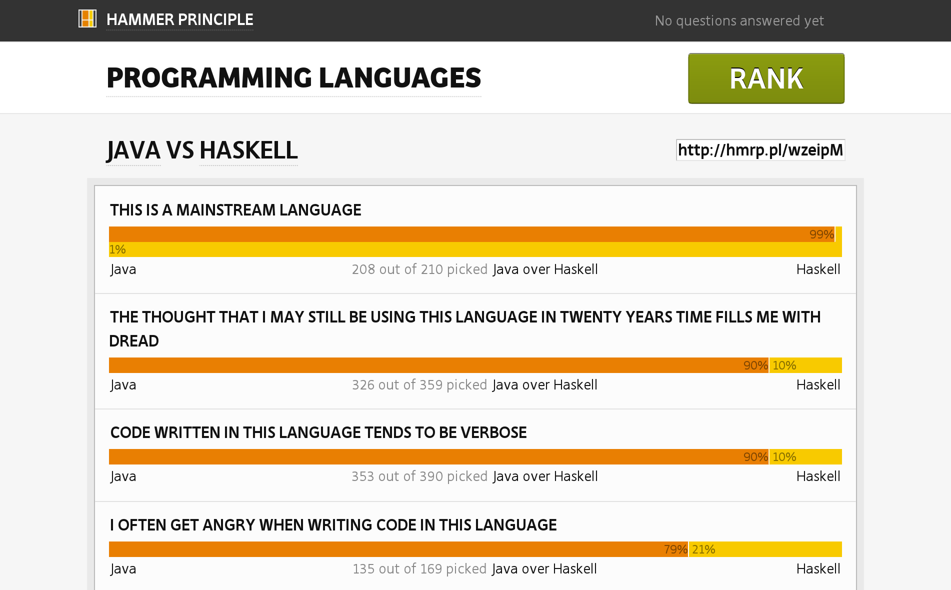Image Source: Hammer Principle

Doesn’t sound that good for Java, what do people say about Haskell?

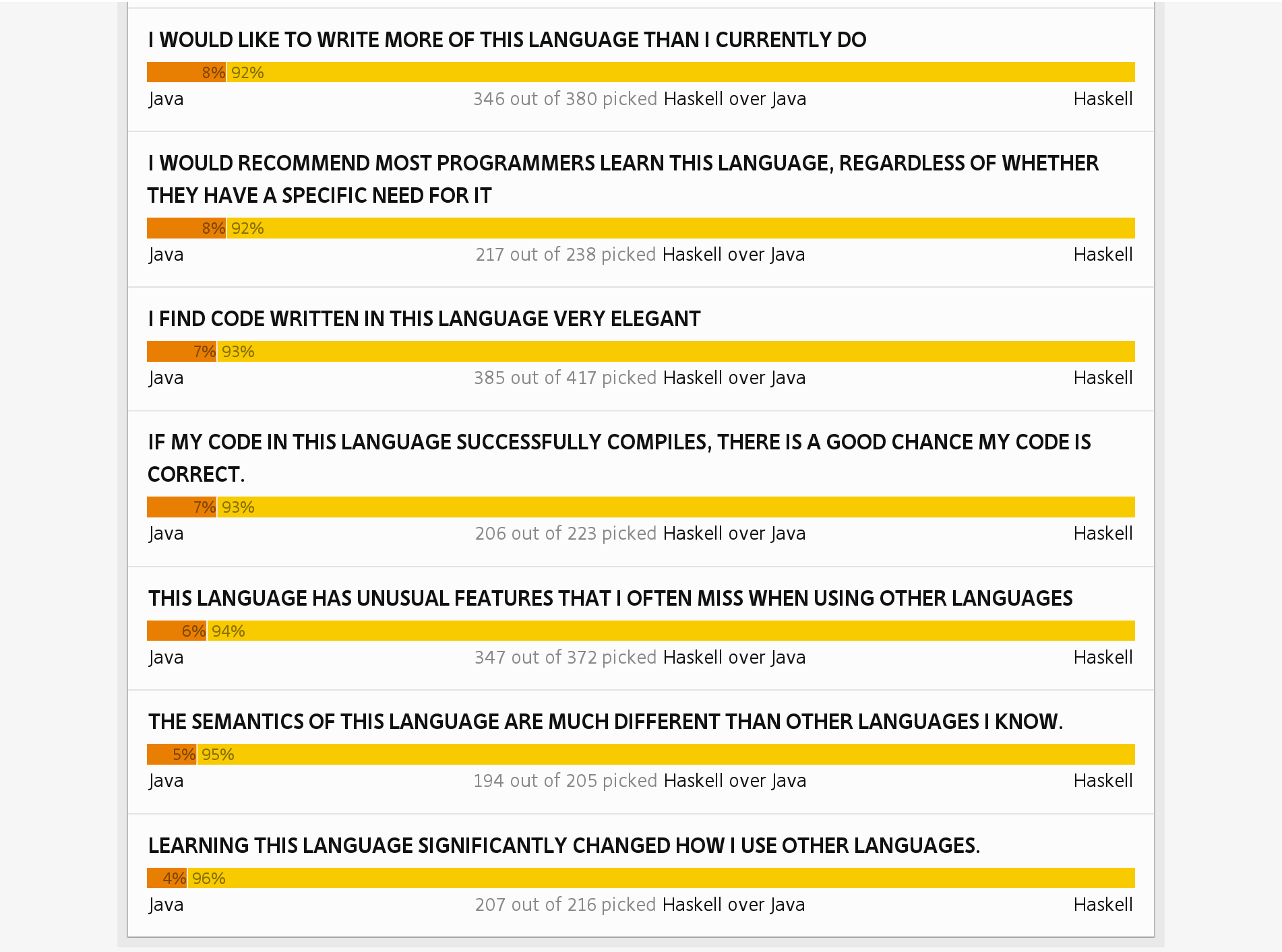Image Source: Hammer Principle

Sounds much better and makes it seem like a reasonable endeavour to learn Haskell! So what is Haskell actually?

Haskell is a purely functional, lazily evaluated, statically typed programming language with type inference.

While this definition sounds complicated you should understand more of it after reading this post. Let’s start with the basics: What’s the difference between an imperative programming language and a functional one? In imperative programming the basic operation is changing a stored value. In functional programming the basic operation is applying a function to arguments.

Haskell itself was designed in 1990 by a scientific committee with the purpose of being a basis for functional programming research. The Glasgow Haskell Compiler (GHC) is the most popular implementation and the one we will be using. You can get it as part of the Haskell Platform as well. Haskell code can be compiled (ghc), but also interpreted (ghci, interactive).

In the rest of this blog post we will look at some key features of Haskell interactively, so you can get your own installation of GHC and follow along and experiment with the code.

Arithmetic

I belive that the best way to learn a programming language is by playing around with it. So that’s what we’re going to do now. I’ll show a few examples and explain the cool Haskell features that we encounter on the way.

We start out by running ghci, the interactive Glasgow Haskell Compiler interpreter (indicated by λ>). We also create a single file tut.hs which we will use to write some more advanced Haskell code and load in the interpreter.

For starters let’s do some basic arithmetic in GHCi, replacing our dusty old calculator:

λ> 2+3
5
λ> 4 * 5
20
λ> 5 / 6
0.8333333333333334
λ> 2 ^ 10
1024
λ> 2 ^ 1000
10715086071862673209484250490600018105614048117055336074437503883703510511249361224931983788156958581275946729175531468251871452856923140435984577574698574803934567774824230985421074605062371141877954182153046474983581941267398767559165543946077062914571196477686542167660429831652624386837205668069376

We see that Integers can be of unbounded size, instead of the usual limits of 32 or 64 bits in many programming languages. Of course if you really want them there are also more efficient machine ints in Haskell:

λ> (2 :: Int) ^ 10
1024
λ> (2 :: Int) ^ 100
0

Using the :: Int notation we specifiy that the number 2 is explicitly of type Int instead of being automatically inferred to be of type Integer. While we’re looking at types, there are also floating point numbers of course:

λ> 2 ** 10
1024.0
λ> 2 ** 1000
1.0715086071862673e301
λ> 2 ** 10000
Infinity

As usual, floating point numbers are of limited precision, so at some point we just reach “approximately infinity”. Let’s do some more math:

λ> pi
3.141592653589793
λ> sin

<interactive>:12:1:
    No instance for (Show (a0 -> a0))
      (maybe you haven't applied enough arguments to a function?)
      arising from a use of ‘print’
    In the first argument of ‘print’, namely ‘it’
    In a stmt of an interactive GHCi command: print it

Looks like sin is a function, but the error message is already confusing. Looking at the part in brackets gives us a good hint: maybe you haven’t applied enough arguments to a function?. Let’s check out the type of sin:

λ> :type sin
sin :: Floating a => a -> a

Invoking :type tells us that sin is a function that takes a value of type a and returns a value of type a, where a is a floating point number. So let’s pass a number to sin:

λ> sin 0.5
0.479425538604203
λ> sin 10
-0.5440211108893698
λ> div 15 6
2
λ> :t div
div :: Integral a => a -> a -> a

div is another function. As you can see it accepts two parameters, both of type a and finally returns a value of type a. In this case a has to be an Integral, some kind of integer-like type. We can even ask GHCi what an Integral is supposed to be:

λ> :info Integral
class (Real a, Enum a) => Integral a where
  quot :: a -> a -> a
  rem :: a -> a -> a
  div :: a -> a -> a
  mod :: a -> a -> a
  quotRem :: a -> a -> (a, a)
  divMod :: a -> a -> (a, a)
  toInteger :: a -> Integer
  	-- Defined in ‘GHC.Real’
instance Integral Word -- Defined in ‘GHC.Real’
instance Integral Integer -- Defined in ‘GHC.Real’
instance Integral Int -- Defined in ‘GHC.Real’

Integral is a type class which requires a few functions to be defined for the type, like quot and rem. We also see that an Integral type needs to have all properties of a Real and an Enum type. Three types are known to GHCi which adhere to this type class: Word, Integer and Int

It looks a bit awkward to write div 15 6, so Haskell offers some syntactic sugar to use the div function in infix notation:

λ> 15 `div` 6
2
λ> 15 `mod` 6
3

The same thing works in reverse to use operators as regular functions, using brackets:

λ> (+) 2 3
5
λ> :t (+)
(+) :: Num a => a -> a -> a

Of course there are quite a lot of other functions that we won’t have time to explore, but you can always explore them yourself in the documentation or using Hoogle:

λ> max 2 3
3
λ> max 5 3
5
λ> 2 > 3
False
λ> not (2 > 3)
True
λ> True && False
False
λ> True && True
True

Lists

Lists are the most important data structure for us, they are simply a collection of values of the same type:

λ> :info []
data [] a = [] | a : [a] 	-- Defined in ‘GHC.Types’
...

What this definition tells us is that a list is a data type that is either an empty list ([]) or a value concatenated with a list itself (a : [a]). So the data type is recursively defined, referring to itself. With this knowledge we can create basic lists ourselves:

λ> []
[]
λ> 1:[]
[1]
λ> 1:2:[]
[1,2]

We can also use some syntactic sugar to create lists instead:

λ> [1,2,3,4,5]
[1,2,3,4,5]

We just said that a list is supposed to be a collection of values of the same type. What happens if we try to break that?

λ> [1,2,3,4,5,True]

<interactive>:27:2:
    No instance for (Num Bool) arising from the literal ‘1’
    In the expression: 1
    In the expression: [1, 2, 3, 4, ....]
    In an equation for ‘it’: it = [1, 2, 3, ....]

Good, that shouldn’t work and indeed it doesn’t. The error message tells us that the list is assumed to be a list of booleans because of the final value. But 1 is not a boolean value, so there is no valid type for this list.

λ> [1..5]
[1,2,3,4,5]
λ> [1,3..20]
[1,3,5,7,9,11,13,15,17,19]

We can store values in variables, but the name “variable” might confuse you a bit, because variables can not be overwritten:

λ> let xs = [1..5]
λ> let xs = [1..6]

The seconds line creates a new variable xs that makes the old one invisible in the new scope. Actually variables are always immutable in Haskell. That means you can easily share access to the same data because there is no way in which it can be overwritten:

λ> let ys = xs

Let’s look at a few common list operations in Haskell:

λ> head xs
1
λ> tail xs
[2,3,4,5,6]
λ> init xs
[1,2,3,4,5]
λ> last xs
6
λ> take 2 xs
[1,2]
λ> length xs
6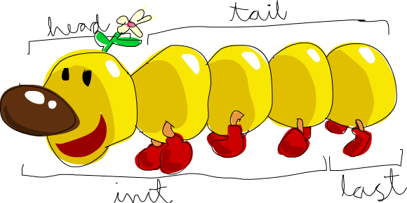

Image Source: Learn You a Haskell for Great Good!

Knowing how lists are implemented we can easily implement our own definitions of these functions:

-- data [] a = [] | a : [a]

head' (x:xs) = x

This definition uses pattern matching. The pattern is (x:xs) where x and xs are variables delimited by the cons (:). We use the knowledge of the definition to split up the passed value into two parts, the first element x and the rest of the list xs. Then the result of our function is simply the first element x.

λ> :l tut
λ> head' [1..5]
1
λ> head' []
*** Exception: tut.hs:1:1-16: Non-exhaustive patterns in function head'

Oops, we didn’t cover one possible pattern, the empty list! We can simply add a definition for that to throw a nicer error message:

head' [] = error "head of empty list undefined"

λ> :r
[1 of 1] Compiling Main             ( tut.hs, interpreted )
Ok, modules loaded: Main.
λ> head' []
*** Exception: head of empty list undefined

Unfortunately there is nothing usefuly we can return for head [], because it’s impossible for us to construct a value of any arbitrary type. Let’s look at the type of head':

λ> :t head'
head' :: [t] -> t

The type was automatically inferred for us, but we can also write it down explicitly if we want to make sure that we don’t break it in the future:

head' :: [a] -> a

This means that head' is a function that takes a list of values of type a as its parameter and returns a single value of type a.

If we had defined head’ for integer lists only, we could return a 0 for example as the default value:

head' [] = 0
head' (x:xs) = x

But if we now check the inferred type we notice that it changed, now only lists containing numbers are supported:

λ> :t head'
head' :: Num a => [a] -> a

So in this case there is nothing better we can do than throw an error.

Analogously we can define the tail function:

tail' [] = []
tail' (x:xs) = xs

λ> tail' [1..5]
[2,3,4,5]
λ> tail' []
[]

This was easy enough. How can we define the last function?

λ> last [1..5]
5

last' [] = error "last of empty list undefined"
last' [x] = x
last' (x:xs) = last' xs

Here the idea is to reduce the problem to something that we can solve. If the list only contains a single element, we know that this exact element is the last one. If the list has more than one element, we remove the first element of the list and recursively call last' on the rest of the list. Yet again the last element of an empty list makes no sense, so we throw an error.

What about defining init? The list of all values but the last?

λ> init [1..5]
[1,2,3,4]

init' [] = error "init of empty list undefined"
init' [x] = []
init' (x:xs) = x : init' xs

The idea here is a bit more complicated. We know that init of a list with one element [x] is the empty list []. If the list has more than one element we know that init contains the first element x, concatenated with init of the rest of the list.

Finally let’s define the length function, which works similarly:

length' [] = 0
length' (x:xs) = 1 + length' xs

The length of an empty list is 0. The length of a list with more than 0 elements is 1 plus the length of the rest of the list. These functions read like mathematical definitions of the properties they are encoding.

Higher-order Functions

So we have defined our first basic functions and noticed that there is no magic happening in Haskell’s standard library. Instead all of these functions are easily implementable. Now let’s look at some more advanced operations that we can perform on lists, for example mapping a function to a list, thus applying it to each value in the list:

λ> let f x = 2 * x
λ> map f [1..5]
[2,4,6,8,10]

It’s a common theme in functional programming to pass functions as parameters to higher order functions. But it’s a bit annoying to define a named function explicitly all the time, so instead we can quickly create an unnamed function, called a lambda function, instead:

λ> map (\x -> x * 2) [1..5]
[2,4,6,8,10]

You can see the lambda function (\x -> x * 2), which is specified to take a parameter x and return x * 2. Of course Haskell has some sweet syntactic sugar to do this even more succinctly by just writing (*2):

λ> map (*2) [1..5]
[2,4,6,8,10]

Let’s see how we can define our own map function:

map' f [] = []

The base case is easy: When we get an empty list passed, the result is also an empty list.

map' f (x:xs) = f x : map' f xs

Otherwise we take the first element x in the list, apply the function f to it and create a new list with this new value as the initial element. We recurse and apply map to the rest of the list in the same way.

At this point we can take a look at the actual implementations in GHC’s standard library and we notice that map is implemented exactly as we wrote it.

Note that we’re not modifying the passed data structure directly, instead we create a new one. Actually in Haskell there is no way to modify data structures, they are all immutable. And functions are pure, so there is no way for a function to have any side effects other than returning a value directly. That’s also why we have referential transparency: When you call a function with the same inputs, it will always return the same output.

Let’s turn to the next function, filter, which keeps only those elements in a list which fulfil a predicate:

λ> filter odd [1..5]
[1,3,5]

Filter is also easy to implement:

filter' f [] = []
filter' f (x:xs)
  | f x       = x : filter' f xs
  | otherwise =     filter' f xs

The guarded equation at the start of the line means that we check a boolean. When f x is true we return the first line, including x, otherwise we don’t include x in the rest of the list. Finally we recurse with the rest of the list, until we reach the base case for the empty list.

By implementing a few functions on list a common pattern emerges. Let’s see how to implement the sum over a list:

λ> sum [1..5]
15

sum' [] = 0
sum' (x:xs) = x + sum' xs

We already implemented the length of a list:

length' [] = 0
length' (x:xs) = 1 + length' xs

How do we define the and function over an entire list?

λ> and [True, False, True]
False
λ> and [True, True, True]
True

and' [] = True
and' (x:xs) = x && and' xs

Notice the similarity by now?

The functions sum, length and and all are built in pretty much the same way. So we can create an abstraction over this pattern, which is called a right-associative fold, or foldr in short:

foldr' f i [] = i
foldr' f i (x:xs) = x `f` foldr' f i xs

Using this pattern it becomes trivial to define these functions:

sum'' xs = foldr' (+) 0 xs

Even better, we don’t need to write down the last parameter, xs:

sum'' = foldr' (+) 0

What’s going on there? Actually in Haskell when you pass a parameter to a function, a new function is returned. So you can consider each function as accepting a single parameter, then returning a new function, which is applied to the next parameter, and so on.

λ> foldr' (+) 0 [1..5]
15
λ> :t foldr'
foldr' :: (t -> t1 -> t1) -> t1 -> [t] -> t1
λ> :t foldr' (+)
foldr' (+) :: Num t1 => t1 -> [t1] -> t1
λ> :t foldr' (+) 0
foldr' (+) 0 :: Num t1 => [t1] -> t1
λ> :t foldr' (+) 0 [1..5]
foldr' (+) 0 [1..5] :: (Enum t1, Num t1) => t1

So in our definition of sum'' we don’t need to have a parameter and put it into foldr', instead we can also have no parameter and just return the function that is returned from (foldr' (+) 0), which takes a list as its parameter.

and'' = foldr' (&&) True
length'' = foldr' (\x y -> 1 + y) 0

We can even define map and filter with foldr:

map'' f = foldr' (\x xs -> f x : xs) []

filter'' f = foldr' go []
  where go x xs
          | f x = x : xs
          | otherwise = xs

Lazy Evaluation and Sharing

While working with lists in Haskell you might wonder what happens if we never reach the base case? We have lazy evaluation in Haskell, which tells us that a data structure is only evaluated when it’s actually needed. So we have no problem handling lists of infinite size:

λ> let x = [1..]
λ> take 5 x
[1,2,3,4,5]
λ> take 5 $ map (*2) x
[2,4,6,8,10]
λ> take 5 $ map (*2) $ filter odd x
[2,6,10,14,18]
λ> x
...

We can even combine multiple infinite lists without any problem:

λ> let y = [1,3..]
λ> let z = zipWith (+) x y
λ> take 10 z
[2,5,8,11,14,17,20,23,26,29]

Of course length won’t work as it will never reach the base case:

λ> length z
^CInterrupted.

Let’s go a step back and create an infinite list of ones:

ones = [1,1..]

The problem is that this is very inefficient, because we recalculate new elements all the time and have to store them in memory.

λ> length ones

You can easily see how the memory usage grows. A more efficient solution is to use recursion in the definition:

ones' = 1 : ones'

We can use ones' itself in the definition of ones', just referring to it. Thanks to lazy evaluation the next value is only evaluated when it is needed, so when we call:

λ> take 3 ones'
[1,1,1]

We see that 1 is the first value of the list, we recurse into ones', we see that 1 is the next value we get, we recurse into ones' and finally we get the last 1.

λ> length ones'

Of course there is no useful result, it’s an infinite calculation, but at least we don’t create a list of infinite size, instead referring to ourselves.

Let’s look at another fun list combinator that takes two lists and creates a new one out of them:

λ> :t zipWith
zipWith :: (a -> b -> c) -> [a] -> [b] -> [c]
λ> zipWith (+) [1..10] [100..110]
[101,103,105,107,109,111,113,115,117,119]

So, zipWith is a function that takes a function (a -> b -> c) as its first parameter. The second parameter is a list of values of type a, the third parameter is a list of values of type b and finally a list of type c is returned.

Of course to understand it we best implement it:

zipWith' f (x:xs) (y:ys) = f x y : zipWith' f xs ys
zipWith' f xs ys = []

We can use zipWith to trivially define a list of all fibonacci numbers:

fibs = 0 : 1 : zipWith' (+) fibs (tail fibs)

λ> take 10 fibs
[0,1,1,2,3,5,8,13,21,34]

The start makes sense, a list of fibs starts with 0 and 1, then the rest is defined with zipWith over fibs itself and (tail fibs). This smells like magic, how can it possibly work? Functions are pure in Haskell. That means that a function always returns the same value when you call it with the same arguments. There is no way to have a variable in which you store some state. Since data structures and functions in Haskell are immutable and pure we can not change them in any way, so we can reuse them without having to recalculate them. So in this case we can refer to fibs' multiple times even inside the definition of fibs' itself.

fibs        0 : 1 : 1 : 2 : 3 : 5 : 8
tail fibs   1 : 1 : 2 : 3 : 5 : 8 :
zipWith (+) 1 : 2 : 3 : 5 : 8 :   :

List Comprehensions

Instead of all these filters and maps we can also use list comprehensions:

λ> map (*2) $ filter odd [1..5]
[2,6,10]
λ> [x*2 | x <- [1..5], odd x]
[2,6,10]

We can even implement the sieve of eratosthenes to calculate all prime numbers as a oneliner with a list comprehension:

sieve (p:xs) = p : sieve [x | x <- xs, x `mod` p > 0]
primes = sieve [2..]

Because in Haskell functions are pure and data is immutable we can perform equational reasoning. We can guarantee that code can be replaced by its definition. Basically this means that you can do refactoring without any risks. You know that nothing can go wrong because there is no state. Every function only takes its arguemnts and returns a value based on those, always the same value. So you can reorganize your functions however you want, the order does not matter and there is actually no order semantically enforced in Haskell.

  primes
= sieve [2..]
= 2 : sieve [x | x <- [3,4,5,6,7,8,9,10,11..], x `mod` 2 > 0]
= 2 : sieve [3,5,7,9,11..]
= 2 : 3 : sieve [x | x <- [5,7,9,11..], x `mod` 3 > 0]
= 2 : 3 : sieve [5,7,11..]
= 2 : 3 : 5 : sieve [...]

Conclusion

I hope you enjoyed this small excursion into functional programming land with Haskell. Maybe you learned something that gives you something to think when programming in your favorite programming language. If you’re interested in learning more Haskell, here are a few books you can read:

Discussions on Hacker News and r/Programming.